Faster warehouse queries don't necessarily require more compute. The strongest query optimization techniques reduce unnecessary work before the engine needs additional capacity, including data scans, materialized columns, joined rows, shuffles, repeated calculations, and resource contention. The practical workflow is disciplined: inspect the plan, identify the dominant cost, make one targeted change, then validate both runtime and resource impact with EXPLAIN or EXPLAIN ANALYZE.

SQL syntax and optimizer behavior vary across Snowflake, BigQuery, Databricks, Redshift, PostgreSQL, and Trino. The examples below are representative SQL or pseudocode, not universal commands. They progress from eliminating data and columns to controlling joins, repeated computation, statistics, parallel execution, and skew. The broader shift toward workload-aware optimization is visible in systems such as Presto, whose history-based framework reuses prior execution statistics for recurring plan shapes, while BigQuery has also introduced history-based optimization using completed executions of similar queries. Presto's history-based optimization documentation describes this move away from static estimates alone.

Querio offers one practical example of warehouse-native, AI-assisted exploration. Its agents and custom Python notebooks can help users generate, inspect, and improve queries, but optimization shouldn't become an opaque automated step. Every recommendation still needs plan validation, correctness checks, and a deliberate production decision.

Table of Contents

• 1. Query Indexing and Index Optimization

  • Validate the access path

• 2. Query Result Caching and Materialized Views

  • Match the acceleration layer to the workload

• 3. Partition Pruning and Time-Series Optimization

  • Confirm elimination in the plan

• 4. Join Optimization and Reordering

  • Diagnose cardinality errors

• 5. Column Pruning and Projection Pushdown

  • Make the projection visible

• 6. Aggregate Push-down and Pre-aggregation Strategies

  • Prioritize by repeated resource use

• 7. Parallel Query Execution and Resource Management

  • Allocate resources by user impact

• 8. Statistics Collection and Query Plan Optimization

• 9. Filter Optimization and Predicate Pushdown

  • Validate where the filter executes

• 10. Data Skew Handling and Shuffle Optimization

  • Match the remedy to the hot key

• 10-Point Comparison of Query Optimization Techniques

• Turn Plan Inspection Into a Repeatable Practice

1. Query Indexing and Index Optimization

Indexing reduces retrieval work by giving an engine a physical path to frequently accessed values instead of forcing a broad scan. That principle is foundational, but traditional indexes don't map cleanly to every cloud warehouse. Snowflake clustering, BigQuery clustering, Databricks Delta data layout, search optimization, and storage metadata can serve a similar purpose even when a conventional B-tree index isn't available.

Start with the workload, not the schema diagram. Look for repeated predicates and join keys in dashboard SQL, generated Looker queries, notebook cells, and recurring pipeline steps. A PostgreSQL reporting database might benefit from a B-tree index on a selective timestamp or foreign key. Other engines may favor composite, bitmap, hash, or partial indexes where supported. A composite structure only helps when its column order matches common access patterns, so an index designed for (account_id, event_date) may not help a query filtering only by an unrelated field.

Validate the access path

Create one structure, then inspect the plan. The validation question is simple: did the engine replace a broad scan with an index seek, a narrower lookup, clustering elimination, or another reduced-read operation?

• Check repeated filters: Prioritize columns that recur in WHERE predicates.

• Check join keys: Examine large joins where the same key appears repeatedly.

• Check write tradeoffs: Indexes and maintained layouts add storage or maintenance work.

• Check actual usage: Remove or redesign structures that the optimizer consistently ignores.

Practical rule: An index that exists but isn't selected by the optimizer isn't an optimization result. It's an unverified hypothesis.

For large fact tables, Snowflake automatic clustering, BigQuery clustering, and Databricks Delta Z-ordering are workload-specific layout choices rather than interchangeable index commands. Test each against representative queries and inspect both estimated and observed scan behavior before deploying it broadly.

2. Query Result Caching and Materialized Views

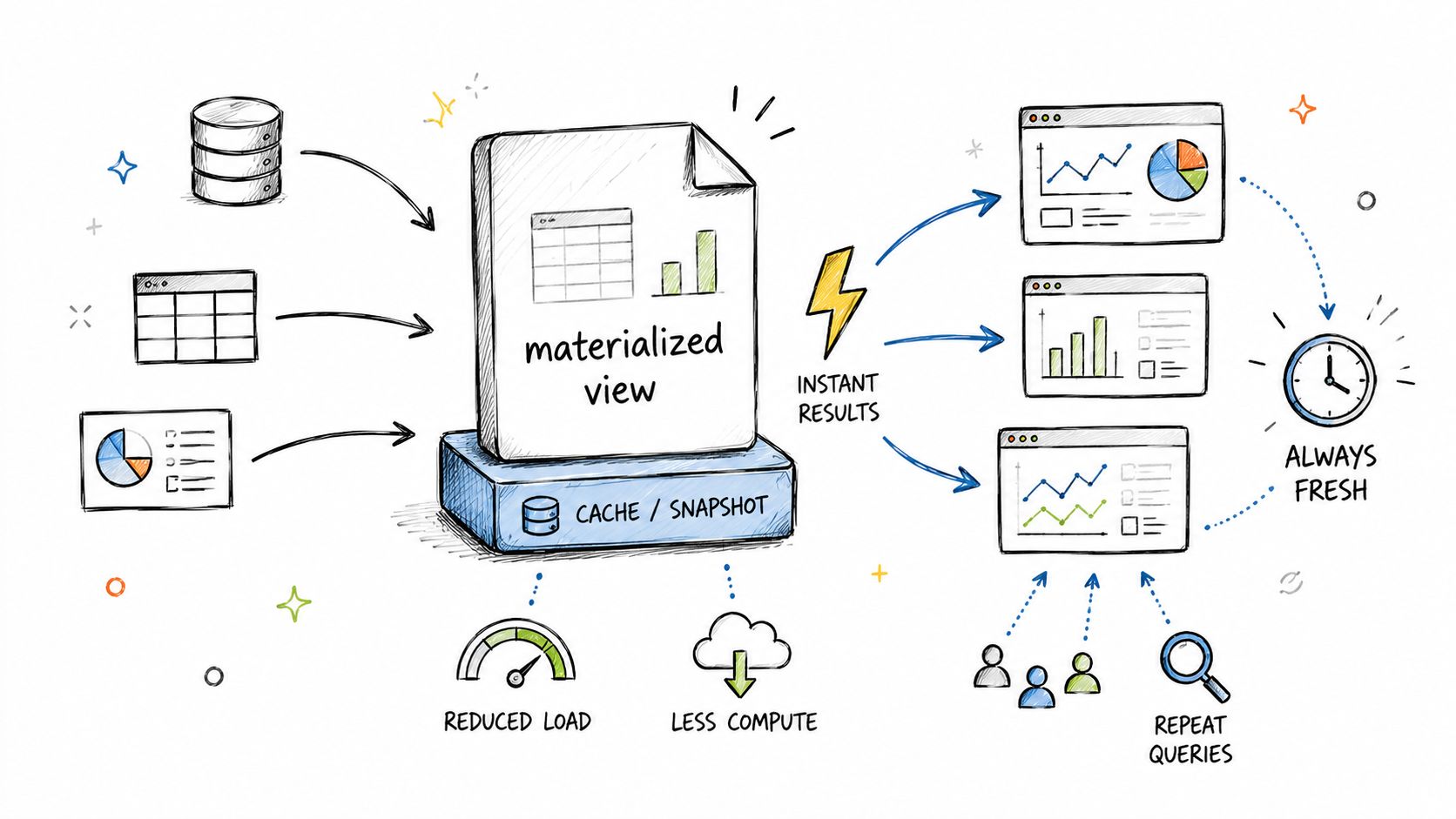
Caching removes computation by serving a result that the warehouse or analytics layer has already produced. A result cache stores an output for reuse when the query and underlying data satisfy the engine's eligibility rules. A materialized view is more deliberate. It persists a transformed or aggregated representation so many related queries can avoid repeating the same work.

That distinction affects freshness and control. A cache hit can disappear after a change in query text, session context, permissions, or source data. A materialized view introduces refresh scheduling, invalidation behavior, storage, and maintenance decisions. For a dashboard that repeatedly asks for the same daily revenue aggregation, a materialized view can be easier to reason about than hoping every request qualifies for a result cache. For interactive exploration, a cache may be appropriate when freshness requirements are looser and query patterns are repetitive.

Match the acceleration layer to the workload

Use EXPLAIN or EXPLAIN ANALYZE where supported, plus warehouse history, to determine whether the query is recomputing its work or receiving an accelerated result. The plan may not expose every cache detail, so pair plan inspection with cache-hit metadata and refresh logs.

• Repeated aggregates: Consider a summary or materialized view when many users ask similar questions.

• Freshness-sensitive data: Prefer live execution or a tightly controlled refresh process.

• Interactive notebooks: Cache stable intermediate cells, but document dependencies.

• Peak usage: Warm known dashboard paths only when the resulting maintenance work is justified.

A practical guide to selecting tools for this workflow appears in Querio's query optimization tools guide. The important operating rule is to document what's cached, what's materialized, and when each representation refreshes. Otherwise, users may mistake an intentionally stale summary for a live source.

3. Partition Pruning and Time-Series Optimization

Partitioning works when the query can prove that whole data ranges are irrelevant. A bounded predicate on a partition column lets the scan eliminate those ranges before reading them. This is especially useful for event, billing, log, and activity tables where users naturally filter by time.

A query such as:

SELECT account_id, event_type
FROM events
WHERE event_date >= DATE '2026-08-01'
  AND event_date < DATE '2026-09-01';

gives the optimizer a direct range. By contrast, applying a function to the partition column can obscure that boundary:

WHERE DATE_TRUNC('month', event_timestamp) = DATE '2026-08-01'

The exact behavior depends on the engine, data type, and optimizer, so don't assume that equivalent-looking predicates produce equivalent scans. Partition grain also has tradeoffs. Daily partitions may suit broad reporting, while hourly partitions can help highly selective operational queries but create more metadata and management overhead. Retention policies and late-arriving events matter too. A partition design that fits append-only data may behave differently when historical records arrive after the original load.

Confirm elimination in the plan

Run EXPLAIN or EXPLAIN ANALYZE and inspect partition counts, file or micro-partition reads, and bytes scanned. If the plan still reads broad ranges, check data types, implicit casts, function-wrapped columns, and whether the filter is applied before a transformation.

• Use stable time predicates: Express ranges directly against the stored partition field.

• Choose grain from access patterns: Don't create fine partitions without selective queries.

• Manage retention: Remove obsolete partitions through an automated process.

• Account for late data: Make backfills and partition maintenance part of the pipeline.

Hash partitioning solves a different problem, namely distribution across workers, and shouldn't be treated as a replacement for time pruning. Querio's explanation of hash partitioning and load balancing helps separate scan elimination from distribution strategy.

4. Join Optimization and Reordering

Joins often become expensive because they multiply intermediate rows, move data between workers, or build structures larger than the optimizer expected. The engine may choose a broadcast join for a small input, a hash join for equality keys, a sort-merge join for sorted or distributed inputs, or a nested-loop strategy for specific predicates. The right choice depends on table sizes, selectivity, statistics, distribution, and memory.

A common mistake is assuming that writing a table first guarantees the engine will join it first. Cost-based optimizers can reorder inner joins, and adaptive systems can revise decisions during execution. Manual SQL still matters because early filters, duplicate control, and clear join conditions improve the evidence available to the optimizer.

Consider:

SELECT f.account_id, SUM(f.amount)
FROM fact_sales f
JOIN dim_accounts a
  ON f.account_id = a.account_id
WHERE a.region = 'West'
GROUP BY f.account_id;

Filtering the dimension before joining may reduce the fact-side work when the engine can push that constraint through the join. It isn't universally beneficial, so validate rather than rely on a rule such as “join the smallest table first.”

Diagnose cardinality errors

Use EXPLAIN ANALYZE and compare estimated versus actual rows at each join. The Join Order Benchmark research demonstrates why complex, correlation-heavy joins expose weaknesses in plan selection and cost estimation. Its benchmark introduced 113 complex join queries, while JOB-Complex evaluates 30 SQL queries and nearly 6,000 execution plans. Those figures describe benchmark design, not a guaranteed production outcome, but they show why simple join-order intuition can fail.

A join that produces far more rows than estimated is a statistics problem until the plan proves otherwise.

Check duplicate keys, null behavior, join type, filtered dimension cardinality, and whether denormalization would remove a repeatedly expensive relationship. Validate the change at the physical plan level, including shuffle volume and spill behavior.

5. Column Pruning and Projection Pushdown

A wide event table can contain identifiers, timestamps, payloads, device attributes, location fields, and nested metadata. A dashboard that needs only an account, date, and measure shouldn't materialize the rest. In columnar storage, selecting fewer columns can reduce the data the engine reads and carries through joins, aggregations, and network exchanges.

The contrast is straightforward:

SELECT *
FROM events
WHERE event_date >= DATE '2026-08-01';

versus:

SELECT account_id, event_date, event_type
FROM events
WHERE event_date >= DATE '2026-08-01';

SELECT * also creates operational risk. A newly added column can increase scan and transfer work, while nested or large text fields may be decoded even though the analyst never uses them. Views and notebook-generated SQL can undermine pruning when they expose or select every field upstream.

Make the projection visible

Run EXPLAIN or EXPLAIN ANALYZE and inspect the scan operator's projected columns. The presence of a narrow outer SELECT doesn't guarantee that storage reads are narrow if an inner view or transformation already requested the full row.

• Name required fields: Treat explicit projections as part of the query contract.

• Inspect nested access: Select only the needed nested paths where the engine supports it.

• Review reusable views: Remove unnecessary wide projections from common models.

• Separate exploration from production: Use broad previews temporarily, not in scheduled dashboards.

Parquet projection pushdown, Snowflake column elimination, BigQuery column pruning, and Spark optimization can behave differently. The plan is the authority for the chosen warehouse, especially when generated SQL comes from a BI tool or AI assistant.

6. Aggregate Push-down and Pre-aggregation Strategies

Aggregation reduces rows, but it can still consume substantial scan, memory, and shuffle resources when performed repeatedly over detailed facts. Push the aggregate into the warehouse rather than exporting raw rows to an application. Then decide whether the warehouse should compute it live or read from a maintained summary.

A live query is usually preferable when dimensions change frequently, users need fresh detail, or the grouping combinations are too numerous to maintain. A pre-aggregated table or materialized view fits recurring metrics with stable grains, such as daily account activity or product-level revenue. Approximate functions can suit exploratory analysis when exactness isn't required, but that choice must be explicit because approximation changes semantics.

Prioritize by repeated resource use

The most useful prioritization rule in the supplied guidance is workload-based: focus on the small share of frequently executed, user-facing queries. One recent optimization guide describes an 80/20 pattern, where about 20% of queries can consume 80% of database resources. That workload-prioritization guidance supports a practical conclusion: a once-a-day report may deserve less attention than a dashboard query executed continuously by many users, even if the report itself runs longer.

Use EXPLAIN or EXPLAIN ANALYZE before and after creating a summary. Confirm that the plan reads the summary rather than the detailed fact table, and compare freshness, refresh cost, result accuracy, and drill-down behavior.

• Choose the grain deliberately: Align summaries with real grouping patterns.

• Preserve drill-down paths: Keep dimensions that users need for investigation.

• Automate refreshes: Make summary maintenance part of the data pipeline.

• Document semantics: State whether metrics are exact, approximate, delayed, or filtered.

7. Parallel Query Execution and Resource Management

Parallelism can shorten wall-clock time by distributing scans, joins, and aggregations across workers. It can also hide an inefficient plan. Increasing warehouse size may make one query finish sooner while worsening queueing, concurrency, or cost for everyone else.

Treat compute as a workload-management decision. Inspect the plan for parallel stages, exchange operators, memory pressure, and spills. Then use execution history to separate queue time from execution time. A query that waits behind other work needs isolation or scheduling attention, not necessarily a rewrite. A query that consumes excessive memory during a hash join may need a smaller input, better filtering, or a different distribution strategy.

Allocate resources by user impact

Snowflake virtual warehouses, BigQuery's managed parallelization, Databricks Photon, and Redshift Spectrum use different controls. Some workloads benefit from autoscaling, while others need predictable capacity and strict concurrency limits. Separate critical dashboard workloads from exploratory or batch work when shared resources create contention.

• Measure queue time: Don't confuse waiting with inefficient execution.

• Use timeouts: Protect shared infrastructure from runaway requests.

• Right-size deliberately: Test capacity changes against representative concurrency.

• Watch spills: Disk spill can indicate a memory or plan problem.

• Retain workload context: Record who runs the query and what depends on it.

Run EXPLAIN or EXPLAIN ANALYZE after resource changes as well as SQL changes. A plan may remain identical while runtime shifts because contention changed, so pair plan evidence with warehouse utilization and concurrency records.

8. Statistics Collection and Query Plan Optimization

Statistics reduce uncertainty about rows, distributions, distinct values, nulls, and selectivity. Microsoft documents how column and indexed-view statistics influence cardinality estimates and choices such as index seeks or scans in Microsoft's optimizer documentation). Oracle recommends collecting base-table statistics through DBMS_STATS.GATHER_TABLE_STATS, with full, sampled, and parallel gathering available. Its DBMS_STATS statistics guidance also provides a basis for automating maintenance.

Start with the estimated-to-actual row comparison in EXPLAIN ANALYZE. A scan that estimates few rows but produces many can push later joins toward the wrong order, distribution, or algorithm. Accurate estimates with broad reads point elsewhere, such as partitioning, clustering, projection, or predicate pushdown.

Use a compact validation loop:

1. Run EXPLAIN to inspect structure, then EXPLAIN ANALYZE where supported.

2. Refresh statistics after major loads, deletes, backfills, or distribution changes.

3. Rerun a representative query and compare estimates, actual rows, and plan versions.

4. Investigate correlated fields, because independent estimates can misrepresent combined filters.

5. Fix estimation errors before forcing a physical strategy.

Statistics age is an operational signal, not a tuning verdict. A changed plan may reflect data churn rather than poorer SQL. AI-generated SQL deserves the same review: inspect its plan, verify that filters and joins match intended semantics, and reject rewrites that improve estimated cost while increasing actual reads or spills. The SQL query optimization resource can help standardize reviews, but engine-native plan evidence must govern decisions.

9. Filter Optimization and Predicate Pushdown

A filter reduces warehouse work only when the scan can apply it early. Predicate pushdown lets a storage connector, file reader, or scan operator discard rows before joins, projections, or aggregations. Columnar formats such as Parquet can use row-group statistics, while distributed engines may apply connector filters or dynamic filters during execution.

Expose the filtered field directly whenever possible:

SELECT account_id, amount
FROM transactions
WHERE transaction_date >= DATE '2026-08-01'
  AND transaction_date < DATE '2026-09-01';

Function-wrapped expressions can prevent partition, file, or row-group pruning:

WHERE DATE(transaction_timestamp) = DATE '2026-08-01'

The appropriate rewrite depends on the schema and engine. A stored date column, an equivalent timestamp range, or a pushdown-compatible expression may preserve the intended result while reducing scanned data. User-defined functions and complex casts require the same check.

Validate where the filter executes

Run EXPLAIN, followed by EXPLAIN ANALYZE where supported. Confirm that the predicate appears at or near the scan, rather than after a broad join or transformation. Compare bytes read, rows produced by the scan, and evidence of partition, file, row-group, or clustering elimination.

Filter partition fields directly and apply predicates before joins when semantics allow. Prefer simple equality and range comparisons, then test more complex expressions against the plan. AI-generated SQL and BI-generated queries often wrap columns in functions, so review both their semantics and their actual scan behavior. Reject a rewrite that looks cleaner but increases reads or delays filtering.

Predicate pushdown applies broadly to columnar warehouses, yet SQL syntax alone cannot prove it worked. The execution plan must show that the engine accepted the predicate and reduced downstream work.

10. Data Skew Handling and Shuffle Optimization

A query can scan little data and still run slowly when one worker receives a disproportionate share of rows. Data skew occurs when a join key, tenant, customer, null value, or time bucket appears much more often than others. The affected task may consume excess memory, spill to storage, or extend the final stage while other workers sit idle.

Diagnose the imbalance in the execution plan before changing the SQL. Check key frequency, partition sizes, task-duration variance, shuffle read and write, spill indicators, and the stage where progress stalls. The remedy depends on the cause. Pre-aggregation can reduce repeated rows before redistribution, while adaptive execution may split or rebalance skewed partitions when the engine supports it.

Match the remedy to the hot key

Salting adds a generated bucket to a heavily repeated key and applies matching logic on the other side of the join. It can spread shuffle work across workers, but it also increases SQL complexity and testing requirements. Use it only when the plan identifies a persistent hot key. Partition hints can help in specific engines, yet forcing a distribution without evidence may shift the imbalance elsewhere.

Run EXPLAIN before the change and EXPLAIN ANALYZE where supported after it. Compare shuffle volume, task-duration variance, spill behavior, peak memory, and final-stage time. Confirm that row counts and join results remain unchanged.

• Profile recurring keys: Skew changes as customer and event behavior changes.

• Pre-aggregate before shuffling: Reduce duplicate rows before redistribution.

• Salt selectively: Limit generated buckets to demonstrably heavy keys.

• Test representative periods: A balanced sample can conceal production skew.

Querio's discussion of negatively skewed distributions can help explain distribution behavior to non-specialists. AI-generated SQL deserves the same review: inspect whether it introduces unnecessary repartitioning, broad joins, or salting without evidence. Keep the rewrite only when the plan shows less contested work and preserved results.

10-Point Comparison of Query Optimization Techniques

Turn Plan Inspection Into a Repeatable Practice

Query optimization works best as a feedback loop, not a collection of isolated tricks. Capture the baseline SQL, parameters, data freshness, concurrency, warehouse or cluster configuration, and user-facing purpose. Run EXPLAIN or EXPLAIN ANALYZE, identify the dominant operator or resource, apply one targeted change, rerun against representative data, and record what changed.

The most important distinction is between reducing work and merely moving it. A larger warehouse may lower elapsed time while increasing contention or resource consumption. A materialized view may accelerate dashboards while introducing refresh lag. A rewritten join may lower row movement but change duplicate behavior if the keys weren't unique. Validation must therefore cover correctness and operational consequences, not only a faster timestamp.

Use this symptom-to-technique mapping as a compact decision aid:

• Bytes scanned are high: Investigate partition pruning, filter pushdown, clustering, and indexing or layout.

• The scan reads too many fields: Apply column pruning and inspect projection pushdown.

• A join produces unexpected rows: Check statistics, key uniqueness, join type, and join reordering.

• The same aggregate repeats: Compare caching, materialized views, and pre-aggregation.

• The query waits in a queue: Review workload isolation, concurrency, sizing, and timeouts.

• Estimated rows differ sharply from actual rows: Refresh statistics before forcing plan changes.

• One distributed task runs much longer: Profile skew, shuffle volume, salting, and adaptive execution.

• A dashboard is frequently reused: Prioritize it over an isolated query when its workload impact is greater.

The evidence should live with the query. Record baseline and post-change runtime, bytes scanned, rows at major operators, spill behavior, queue time, concurrency, freshness, and cost where the platform exposes those measures. Also record the reason a change was rejected. An unused index, an unnecessary summary table, or a risky hint creates maintenance burden without reducing production work.

AI-assisted tooling can shorten the investigation cycle. An agent can propose a predicate rewrite, identify a wide projection, surface an estimated-versus-actual row anomaly, recommend a cache or summary candidate, and generate notebook experiments. For natural-language and agent-generated queries, this is increasingly important. A 2026 survey of LLM query optimization organizes methods around expansion, decomposition, disambiguation, and abstraction, which frames optimization as a system-design problem rather than a narrow SQL style exercise.

Human review remains essential. People must confirm metric definitions, permissions, data freshness, join semantics, sensitive-field handling, and production rollout conditions. AI can make the hypothesis stage faster, but EXPLAIN ANALYZE, representative data, and accountable ownership decide whether a recommendation is safe.

Querio's warehouse-native AI agents and custom Python notebooks provide one way to make this loop accessible to technical and non-technical users. They can help users explore company data, inspect queries, and turn promising experiments into reusable self-service workflows without removing the plan-validation discipline that keeps analytics trustworthy.

Make query optimization a measured operating habit, not a last-minute response to a slow dashboard. Use Querio to explore warehouse data with AI agents and custom Python notebooks, then inspect and improve the resulting queries with a clear feedback loop. Visit Querio to give both analysts and business users a practical path from question to validated warehouse decision.